מפל מתח בכבלים ארוכים

Define the two measurement points

Voltage drop describes a difference between specified points. Name the sending point and the receiving point before calculating. “Workshop board to store board” is a useful description. “The installation loses three volts” is incomplete unless the reader knows which installation section, which current and which voltage reference are involved.

Distinguish supply voltage variation from a calculated cable drop. If the voltage at the workshop board changes, the store's receiving voltage changes even when the cable and load stay the same. A cable calculation alone does not describe the entire range of operating voltages that equipment may experience. Keep the assumed sending voltage visible in the example.

For the first exercise, assume a single phase 230 volt supply, a 60 metre one way route and a 12 ampere steady load with unity power factor. Assume each conductor has a resistance of 4 ohms per kilometre at the chosen operating condition. Ignore reactance in this simplified resistive calculation. Each assumption defines the model rather than a universal installation rule.

Avoid doubling the route twice

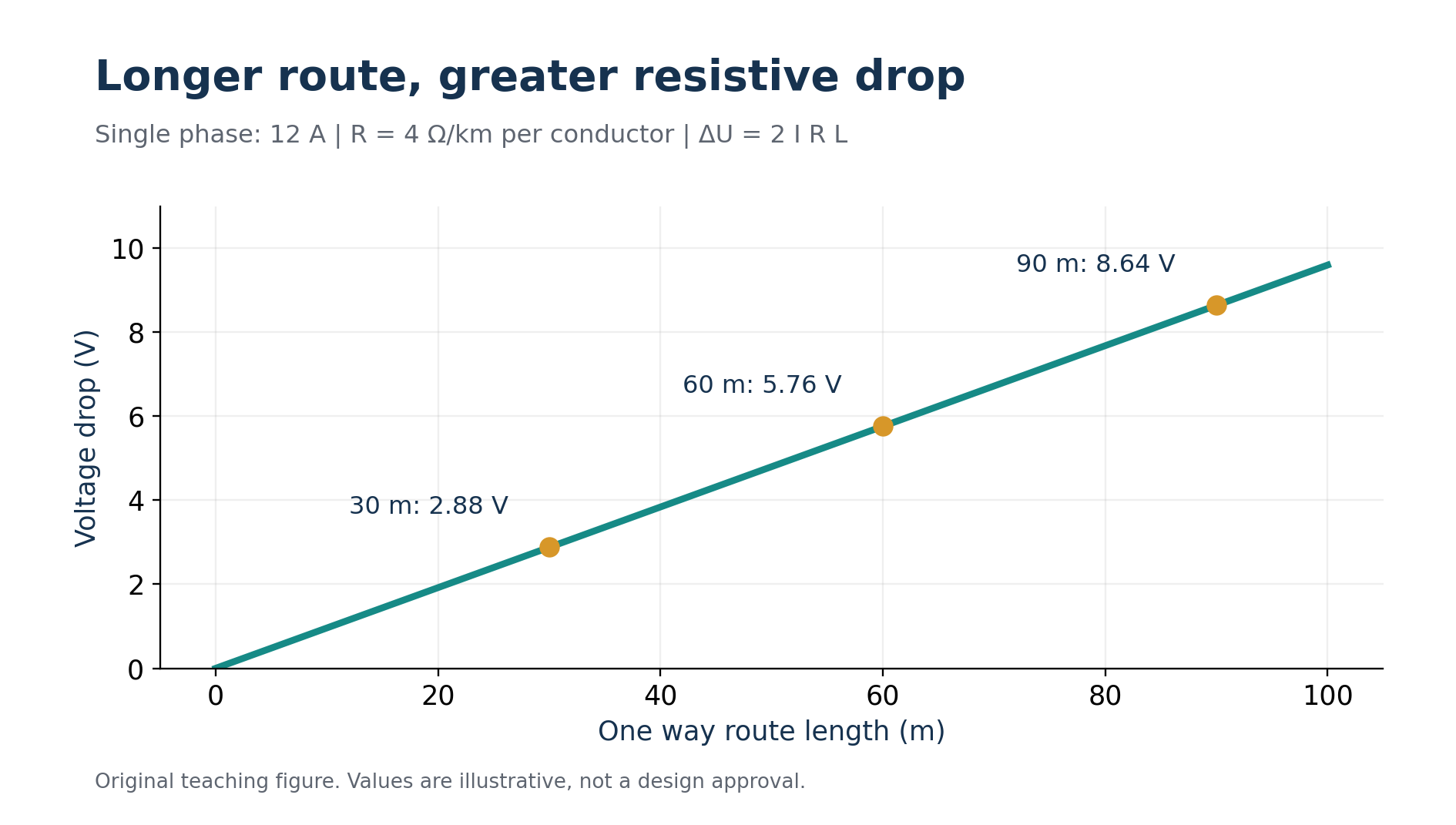
In a two conductor single phase circuit, the current travels to the load and returns through the other conductor. A simplified resistive expression is ΔU = 2 × I × R × L, where R is the resistance of one conductor per kilometre and L is the one way length in kilometres. The factor of two already accounts for both conductors. [2]

Convert 60 metres to 0.06 kilometres. The drop becomes 2 × 12 × 4 × 0.06 = 5.76 volts. Relative to the assumed 230 volt sending value, that is 5.76/230 × 100, approximately 2.50 percent. The calculated receiving value is 224.24 volts under the simplified assumptions.

If somebody enters 120 metres and also retains the factor of two, the result doubles incorrectly. Another common error is using a resistance already stated for the complete loop and multiplying by two again. Read the data heading, not just the number. Ask whether the resistance describes one conductor, a pair, or a complete measured circuit.

Length units matter just as much. Using 60 with a resistance in ohms per kilometre produces a result a thousand times too large. Put the conversion beside the equation. A reader should be able to identify the length convention without guessing how a spreadsheet cell was formatted.

Understand what changes the result

In this simplified model, voltage drop changes in direct proportion to current and route length. At 6 amperes, the fictional run loses 2.88 volts. At 18 amperes, it loses 8.64 volts. Doubling the current doubles the calculated drop because the assumed resistance and route remain unchanged.

Now keep 12 amperes but compare route lengths of 30, 60 and 90 metres. The corresponding drops are 2.88, 5.76 and 8.64 volts. This comparison shows why a small load can still require a careful assessment when its supply path is long. It also gives an intuitive check on a calculator output.

Resistance changes the result too. If a different candidate has an assumed resistance of 2.5 ohms per kilometre under the same conditions, the 60 metre calculation becomes 3.6 volts, approximately 1.57 percent. The improvement comes from the changed resistance. It does not establish that the new candidate satisfies thermal capacity, mechanical suitability or protective requirements.

Use the resistance associated with the relevant conductor material and temperature basis. A room temperature value and a value representing a warmer operating conductor are different inputs. If a tool uses a particular manufacturer data set, identify that basis when comparing its output with another calculation. Two different assumptions can explain a disagreement without either arithmetic operation being wrong.

Include power factor and reactance when required

For a single phase AC calculation with the appropriate impedance model, the expression becomes ΔU = 2 × I × (R cos φ + X sin φ) × L. For a balanced three phase circuit, the corresponding factor is √3 rather than two. Schneider Electric's guide sets out these relationships and the associated voltage references. They are approximations within their stated steady load models. [2]

Take a second fictional example: a balanced 400 volt three phase feeder, 100 metres long, carrying 25 amperes. Assume R is 1.2 ohms per kilometre, X is 0.08 ohms per kilometre, and cos φ is 0.8. With the stated sinusoidal assumption, sin φ is 0.6. The combined term is 1.2 × 0.8 + 0.08 × 0.6 = 1.008 ohms per kilometre.

The calculated line to line drop is √3 × 25 × 1.008 × 0.1, approximately 4.36 volts. Its percentage is 4.36/400 × 100, approximately 1.09 percent. Use the 400 volt line to line reference because that is the voltage represented by this balanced three phase calculation.

Do not swap the single phase and three phase multipliers based on whichever produces a preferred answer. Establish the circuit arrangement first. Similarly, do not use cos φ as a substitute for true power factor without considering waveform conditions. A problem involving strongly distorted currents may need a different or more detailed assessment than this teaching model.

Account for the complete relevant path

The store example may include an upstream feeder before the workshop board. Suppose a simplified analysis assigns that feeder a 3 volt drop under the same stated operating scenario, while the final run contributes 5.76 volts. The cumulative reduction is 8.76 volts when the values refer to compatible voltage quantities and conditions.

The compatibility condition is important. Do not casually add a line to line three phase result to a phase to neutral single phase result. Do not add drops calculated at unrelated peak currents that cannot occur together and call the sum a verified operating case. Define the scenario and voltage reference before combining section results.

A useful record starts with a one line route map and lists each section's length, current, model and calculated drop. It can then show the cumulative value at each board. This makes it easier to identify where a redesign will have the greatest effect, especially when a long upstream section supplies several downstream circuits.

Compatible upstream and final circuit drops add to 8.76 volts in this fictional operating case. Original chart.

Establish the applicable permitted limit from the relevant Israeli requirements and project conditions. An international guide can explain a calculation method without establishing the local legal criterion. Avoid presenting a familiar percentage as a universal pass mark. The criterion and its source belong beside the calculation, not in an assumption hidden at the end.